Welcome to the second edition of Trent's Bayesian Bank! After exploring Gaussian processes for non-Gaussian likelihoods last time, we are going to take a look at some time-series modelling in this instalment. Specifically, we are going to see how well a stock-standard model straight from the Stan (probabilistic programming language that fits Bayesian models) documentation can recover the parameter values we set on some simulated data using an autoregressive moving average (ARMA) model. Let's jump in!

Quick introduction to autoregressive moving average models

Autoregressive moving average (ARMA) processes are a highly common type of time series. They are composed of the sum of a constant term, an autoregressive (AR) component, and a moving average (MA) component. Let's break that down to understand the components properly before we take a look at the whole thing.

AR models essentially aim to predict future values from past values of a series at some time lag denoted p, with some coefficient denoted phi and with some error epsilon. Mathematically, this can be expressed in the following way:

AR processes are seen in all kinds of fields, including statistics, finance, economics, and medicine. Importantly, most AR models assume stationarity of the time series; that is, the mean and variance are equivalent along the series and there are no periodicities or seasonality present. If our data is non-stationary, we typically need to difference or transform the data to enforce stationarity. More precisely, an AR process with an absolute value of phi >= 1 is non-stationary. We'll touch on this later when we build our model.

MA processes are also commonly encountered as they describe data which can be predicted from some historical and current coefficient and error term. We can write it mathematically as:

Taking both the AR and MA components together, we can compose the full ARMA model using a sum. This now gives us the following equation for the full ARMA process:

Very cool! Let's now simulate some data from such a process and get started.

Simulating some data with specific parameters

Simulation is absolutely one of the most important tools in any analyst's bag. In this case, we can use simulation to specify an exact statistical process with specific parameter values. Because we know the parameter values, we can use this knowledge to assess the performance of models in estimating these values purely from the data. Here we are going to simulate some data from an ARMA process with an AR coefficient (phi) of 0.8 and an MA coefficient (theta) of 0.2. We can do this in R with the following code while also drawing a plot of the data and loading the packages we need for the entire analysis:

Nice. It looks like a textbook ARMA process with no evident trend, periodicities or other non-stationary aspects (as we expect). Let's take a look at how we can build a probabilistic model to try and estimate our parameter values for this particular process.

Specifying a Bayesian ARMA model in Stan

Time to write some Stan! At a high level, Stan is a probabilistic programming language written in C++ (meaning we must use C++ conventions too) that is a state-of-the-art tool for fitting Bayesian models using Markov chain Monte Carlo (MCMC). A Stan model is composed of multiple named chunks (for a more detailed discussion on what goes into each Stan chunk, please see the previous Trent's Bayesian Bank post). We are going to use an ARMA model straight out of the Stan documentation here to see how well it does. The Stan model looks like:

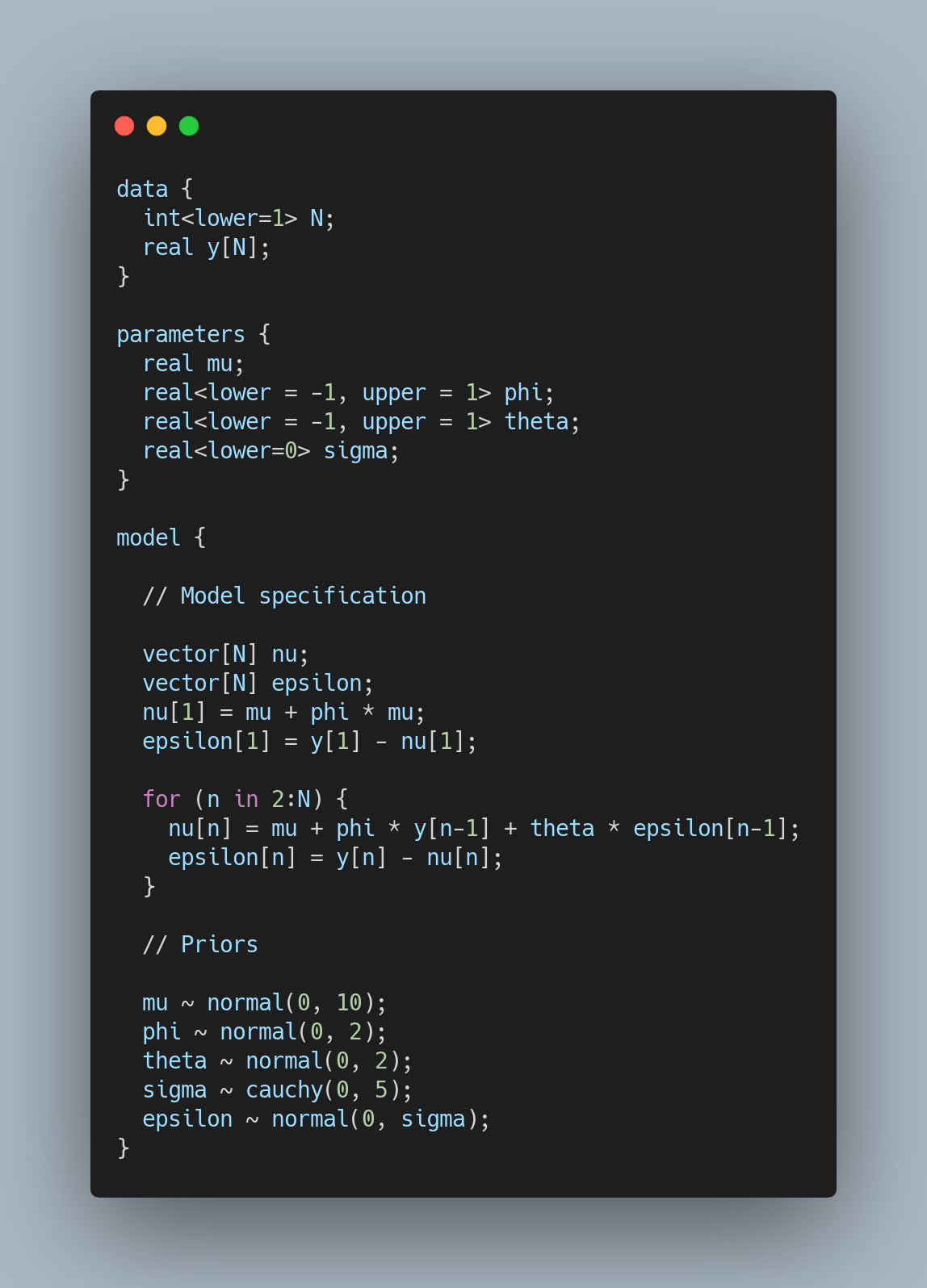
Let's break down each component so you know exactly what it's doing.

data

This is where any inputs we supply to Stan go. Here we are only defining the sample size N and the values themselves y. Note that we fix the lower bound of N as we can't have less than one observation.

parameters

This block is where declare variables that the Stan program will estimate. We are declaring a constant \mu, our AR and MA coefficients \phi and \theta respectively, and the standard deviation of our error distribution sigma. There are two things to note here. First, we fix the lower bound of \sigma to zero as we cannot have a standard deviation of less than zero. Second, we fix the range of both \phi and \theta to be between -1 and 1. This has two core benefits:

1. It ensures that the generative model we build is stationary
2. It ensures numerical stability as values above 1 or below -1 can seriously interrupt the MCMC process resulting in extremely long fitting times (seriously, remove these bounds and re-run the model and see how long it takes compared to ours here!)

model

This block is where we define our priors and the sampling model. Let's start with the priors first. You can see we are placing probability distributions (priors) over all of the parameters we defined in the previous block with the addition of one more-- epsilon, which governs the error between our model predictions and the actual data. We don't know how "wide" this distribution might be, hence why we are estimating its standard deviation \sigma as part of the program. The other parts of this block pertain to sampling. You might note from the outset that this code looks somewhat familiar--which it is! It looks pretty close to the equations I presented for an ARMA model earlier. This is a good thing, as we are essentially specifying the ARMA process from scratch here using probability distributions! The close relationship between math and code is one of the things that makes probabilistic programming so flexible and rewarding.

We are instantiating the first entry in our storage vectors for our model predictions (nu) and error (epsilon) outside the for loop as we clearly have no lag value to use the formula for. So we simply instantiate index one for nu as the constant plus our AR coefficient multiplied by it. This ensures our model prediction is in the ballpark of the raw data (think of Apple's stock price compared to an ARMA process with a mean of 0). Our error at index one (and all indices for that matter) is of course the predicted value subtracted from the actual value.

With our model specified, we can fit it in R with the following:

For a Bayesian model fit using Markov chain Monte Carlo (MCMC), this actually fits pretty fast! This is in part because our input data isn't large, but also has a lot to do with the fact we purposefully restricted our core parameters of \phi and \theta to values that define a stationary series.

So how well did our uninformed, stock model perform? Let's extract the posterior distributions and plot them against the true values we simulated our data with. We can make use of the excellent ggdist package for nice distributional graphics on top of ggplot2.

Pretty interesting! Our model successfully recovers the true parameter values with both 80% and 95% probability! However, you will note that the true AR coefficient (\phi) value is not aligned with the general area of highest probability density (nor the median) from our posterior distribution. While our credible interval does contain the true value, we would ideally like to see a stronger alignment between the region of highest probability density with the true parameter value. This could be a byproduct of us just fitting a stock model with no cogent thought on priors, but it's still pretty interesting that such a model can recover the true value with 80% and 95% probability.

For the MA coefficient (\theta), we can see a close alignment between the general region of highest posterior probability density and the posterior median with the true parameter value. Very nice!

Final thoughts

Thanks for making it to the end! I hope you found this short piece somewhat informative. Probabilistic modelling is an incredibly powerful tool and the flexibility to parameterise every component of a model with probability distributions can lead to informative work on understanding the underlying generative processes of various real-world and synthetic data.