Welcome to the tutorial! In this short piece we are going to explore robust regression estimators and how they can be used to address violations of the homoscedasticity assumption of linear regression. All R code to reproduce the outputs is presented throughout.

Heteroscedasticity

Heteroscedasticity is a big word that essentially just means "non-constant variance" or that the variance of our y value varies as a function of the variable(s) that predict it (i.e. x). On a bivariate scatterplot, heteroscedasticity is usually visible as a "fanning" shape as we move along the x axis. We can see this in the plot below.

The code below generates the plot.

library(dplyr)
library(magrittr)
library(ggplot2)

# Simulate heteroscedastic data

set.seed(123) # Fix R's RNG
n <- 1000 # Sample size
x <- seq(from = 1, to = n, by = 1) # x variable values
sd <- runif(n, min = 0, max = 1) # SD of error
epsilon <- rnorm(n, mean = 0, sd = sd*x) # Non-constant error
y <- x + epsilon # y values from linear predictor

# Plot

tmp <- data.frame(x = x, y = y)

tmp %>%
  ggplot(aes(x = x, y = y)) +
  geom_point(size = 2) +
  geom_smooth(formula = y ~ x, method = "lm")

Diagnosing heteroscedasticity

The presence of heterscedasticity is typically assessed graphically using a residuals and/or standardised residuals plot from a linear model, though we can usually (if the dataset is small enough) initially infer its presence from bivariate scatterplots as seen above. A model with homogeneity of variance should have no discernible pattern across the fitted values as a function of standardised residuals. This plot is depicted in the bottom left of the matrix of graphs below. The following R code generates that example.

mod <- lm(y ~ x, data = tmp)

par(mfrow = c(2, 2))
plot(mod)

Note that this model clearly violates other core assumptions of linear regression but we won't be discussing those here.

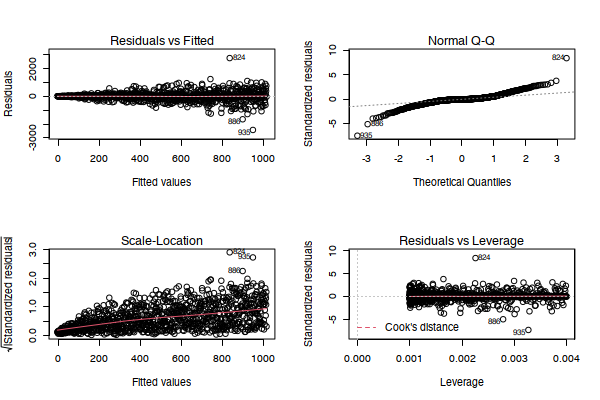
Evidently, there is a non-horizontal line through the plot, and the fanning shape is particularly visible, indicating heteroscedasticity. We can confirm this hypothesis through a follow-up numerical assessment known as the Breush-Pagan test. If the Breush-Pagan test is statistically significant, then we have further evidence that our data is affected by heteroscedasticity. Note that this approach of "building evidence" is extremely important in statistics - it is often the case that one test is not sufficient to make a claim, so building a case through multiple assessments can be a rigorous way to inform your decision making. This test can be implemented in a single line of R code:

library(lmtest)
lmtest::bptest(mod)

Our resultant p-value is much less than any of the traditional cut-offs of .05, .01, and .001, which strongly supports our case for the presence of heteroscedasticity.

Tools to handle heteroscedasticity

Now that we have confirmed the presence of heteroscedasticity, we can begin looking at our options. Typically, most people would opt for one of the following:

• Quantile regression
• Weighted regression
• Robust variance-covariance estimators
• Nonlinear model

While each of these tools are useful in their own right, this tutorial will only consider the robust variance-covariance estimator option.

Robust estimators

Before we get into the mechanics of robust estimators, let's quicky revisit the structure of an ordinary least squares (OLS) regression model. Remember that in linear regression we are trying to model a conditional mean with some error around it (hence why we assume normality in OLS regression, as a mean and standard deviation completely parameterises a normal distribution). We are all familiar with the classic form:

Where our linear predictor is comprised of the intercept, regression coefficient, observed X value(s) and the error term - as noted in the equation. However, mathematically, this form does not explicitly tell use how to solve the regression equation to derive the coefficients, intercept term, and error estimates. Instead, we can write the regression equation in its matrix form to show exactly how the vector of coefficients are calculated:

In plain words, we are computing the product between the transpose of X and X itself, taking the inverse of that, and then multiplying the result by the transpose of X and Y. If it's been a while since you studied statistics, this might be how you are feeling:

Now, robust estimators introduce some spice to this equation by adding some "meat" between the existing "bread" of the matrix form regression equation (this is why statisticians refer to robust estimators as a regression "sandwich"). This "meat" is typically referred to as Omega and in the context of the full equation looks like this:

Omega flexibly acts on the diagonal of the variance-covariance matrix, and relaxes the assumption of homogeneity by enabling differing variances along the matrix diagonal. In practice, the inclusion of heteroscedastic-robust estimators reduces the size of test statistics, drives significance values away from zero, and increases standard errors to reflect the variance structure of the data. There are several different types of Omega that we can choose from. Statistical software usually denotes these numerically as different "heteroscedastic-consistent" (HC) options:

• HC0
• HC1
• HC2
• HC3
• HC4

For quite a lot of datasets, each of these options usually return quite similar results, and so the default HC3 option specified by the authors is usually recommended. This is because HC3 has been shown to give the best performance on small samples as it weights influential observations less than other options (though HC1 and HC2 also perform decently on small samples). HC0 is argued on the basis of an asymptotic nature and HC4 is a more recently proposed alternative to HC3 that may perform even better in the presence of influential observations. For the sake of brevity, I will only present the mathematics of HC3 as that will be our focus today (see here for details on the others):

In this equation, u represents our model errors and h represents the diagonal elements of the hat matrix - which describes the mapping of the y variable values to our predicted y-hat values. In comparison, the standard OLS assumption would have a w weight vector described by:

Where each element of the matrix diagonal receives the same variance - which is consistent with the standard modelling assumption we all know. Robust estimators are implemented in R using the aptly named sandwich package. We can adjust our initial OLS estimates with a minimal amount of additional code by simply calling the robust estimation on our regression model object. The sjPlot package provides some nice auto-formatted tables to view outputs:

library(sandwich)
library(sjPlot)

tab_model(mod, vcov.fun = "HC", show.se = TRUE)

I find it useful to compare the standard errors (SE), t-statistics, and p-values from the original model outputs and the heteroscedastic-consistent adjusted outputs to fully understand the extent of the correction. The original model's outputs can be accessed in a single line of code:

summary(mod)

Concluding thoughts and additional resources

Thanks for making it this far! I hope you found this a useful overview and feel motivated to learn more or implement robust estimators in your own work. If you are interested in diving deeper, here are some useful resources:

• Linear Models with R
• sandwich R package
• A Matrix Formulation of the Multiple Regression Model